Summing Up Clustering

1. Overview

Clustering algorithm types

All types
│———Prototype Based: point assignment
│   |   
|   |———Centroids: distance metric applied to center of a subgroup
|   |
|   |———Medoids: representative point of the graph  
|
└─── Hierarchical Based
│   │
│   │———Agglomeration
│   │
│   └───Division
│   
└───Density Based

2. Agglomerative algorithms

Agglomerative algorithms start from singletons, and they differ because of the strategy used to merge 2 clusters, i.e. the metric used to calculate the distance between 2 clusters. Let’s see different strategies of merging clusters.

• Single Link(MIN): find all min distance between any 2 points from two clusters, and compare. Min(min(2clusters))
  Time complexity O(n^2), we do not need to recompute the pairs each time.
• Complete Link(MAX/CLIQUE): find all max distance between any 2 points from two clusters. Min(max(2clusters))
  Time complexity O(n^2 log n), consider the first merge, compute each pair & sort.
• Group Average: keep updating the centroid of each cluster. Min(d(2centroid))
• Ward’s Method: track the increase in squared error when merged. Min(Increase_SE(2clusters))

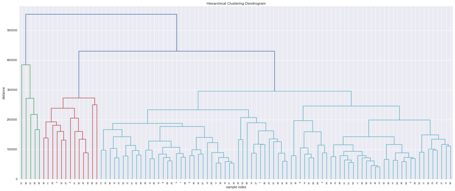
Real example from the retailer data:

3. Divisive algorithms

Interestingly connected with MST, just consider the whole graph made up of weights(distance between 2 clusters), first find the MST, and break link corresponding to the largest distance.

4. K-means: A better start

When Initializing k centroids, we’ll not do it randomly, instead:

Pick one point randomly into the active set s while len(s) <k, add a point whose minimum distance from s is maximized.

Then we’ll follow the normal process, assign each point to the nearest centroid & update the centroids. Note that the global minimization function is min(SSE) = sum(sum(SSE each cluster))

5. Find the best k?

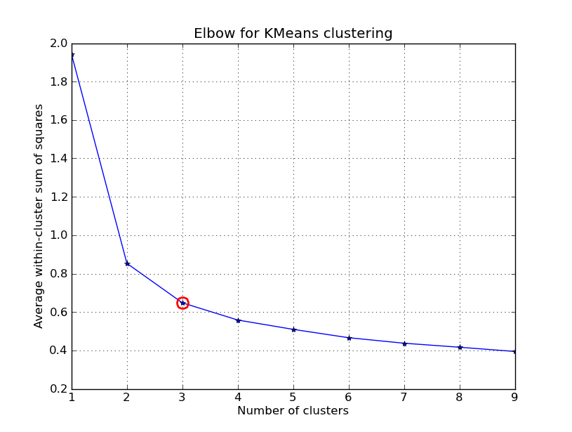
Elbow Method – graphically.

Note: this is typically used in K-means for the case that K is unknown, but in the implementation of the algorithm, we shall assign a K value in advance. (Q: We can also use it in Hierarchical?)
For Hierarchical clustering, the process can stop when there’re a fixed number of clusters left, or we can stop until there is no further compact merge, which means we need to define a threshold for the merged diameter/radius.

6. Some thinking

• Hierarchical clustering is relatively fast because of its greedy nature, the process is very much like constructing a Huffman tree. However, we don’t have a global objective function, which means in each merge decision, it’s not made from a globally optimized point of view, the resulting clusters are not even stable. I think this is the key difference distinguishing it from k-means.

• Computation complexity for hierarchical clustering:

  In the basic setting, obviously it’s O(n^2)+O((n-1)^2)+O((n-2)^2)… = O(n^3)
  Now introduce a improved one: initial step: O(n^2), Form the pairs into a priority queue (constant time to find pairs to merge), which takes O(n^2). Here’s the trick: when decide to merge C & D, remove from the priority queue all entries involving C or D (Deletion O(log n), at most 2n deletions). Recompute the pair distance and insert (O(log n) for insertion, and at most n insertions). Thus, overall it’s O(n^2)+O(n^2)+O(n*nlog n)=O(n^2log n).

• Computation complexity for K-means:

  Global optimization function NP Hard. The running time of Lloyd’s algorithm is naively O(nkdi), where n is the number of d-dimensional vectors, k the number of clusters and i the number of iterations needed until convergence.

• Ward’s method can be used as a robust method of Initializing a K-means clustering.