- This work is under guidance of Professor Saravanan Kesavan in UNC Kenan-Flagler Business School.
Given a retailer’s data across 123 stores through 47 weeks, we want to apply the Newsvendor model to estimate service level for managers in each store. Further research will be, to discover what kind of factors are affecting manager service level.
1. Newsvendor Model General Summary
E[Profit] = E[p*min(q, D)-cq]
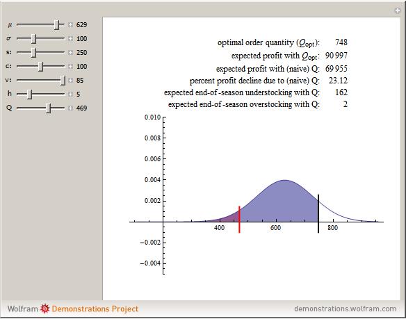
Here c, p is the fixed cost and price for each unit of demand, q is the number of units stocked(q* will be the best decision we make about inventory amount, it is what we’re interested in). D is a random variable with CDF F representing demand.
The solution q satisfy: F(q)= (p-c)/p
Starting from the very basic case above, in our research, the newsvendor problem assumes only overage and underage costs (denoted C_o and C_u, respectively). It’s not hard to see that C_o ~ c, C_u ~ (p-c). Thus F(Q*)=1/(1+C_o/C_u). The ratio is referred to as “Service Level”.
- Notes: Derivation of the result. Take the expectation of the loss as our objective function L, we want to minimize it. Let Q be the inventory amount, x is the real demand.(R.V.). Then the loss will be:
- l1(Q, x) = (Q - x)C_o, if x<=Q
- l2(Q, x) = (x - Q)C_u, if x>Q
Now the objective function is L(Q) = Int_x_0_Q( l1(Q, x)*f(x) ) + Int_x_Q_inf( l2(Q, x)*f(x) ), let L’(Q) = 0, we will get the result shown above.
2. How We’ll Apply the Model
Different from direct application, a twist in this research is that we’re interested in the “best labor spend”(i.e the money spent on labor) for each store, rather than the inventory amount. In the standpoint of a store manager, similar to inventory, overly or underly arrange the labor than the real need will bring loss. Therefore, the service level of a manager measures his/her labor arrangement strategy.
For each week, the labor_goal column in the data refers to the labor cost planned to be made based on the actual sale data, and actual_labor refers to the actual optimized labor cost L*. Thus, if we can get the labor cost distribution F(l), given the known L*, we can calculate the service level directly.
Now problem comes to how can we find the labor cost distribution? The idea is, given that we’re able to find the demand distribution, and if we know some relationship between the demand distribution and labor distribution, then we can find the labor distribution as well. The connection here is made by Budget Function, it takes the actual labor as input and labor goal as output. This function is a measure of “how much you should have spent on labor” given the actual sale.
- Notes: Demand is completely measured by sale, thus we’re not distinguishing the two concepts. Demand is a random variable, and we’re assuming demand ~ sale forecast + random noise, thus we’re going to find the pattern of random noise in the first place. The sale forecast is measured by the sales_manageradj column.
3. Steps To Go
- First thing to do is finding the demand distribution F(x) for each store.
- Given the labor_goal data, and sale data, find the labor budget function B.
- Using demand distribution + budget function, get the labor distribution F(l)
- Using the given L* to find service level for each store(manager).
- Find factors that affect the service level.

