Demand Distribution

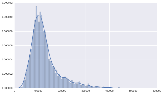
Number of Data Points to Estimate?

Overall, it’s very well normal-shaped, with a little bit “long tail”.

sns.distplot(df_demand['actual_sales'].values,bins=100)

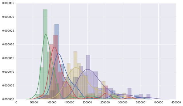
But divided them into stores, take first 5 as example, we’ll find their shape has a lot variation.

Now think about our logic: we’re not assuming the actual-sale value is normally distributed, which is a too strong assumption. Instead, we’re assuming the “error of plan”: (actual_sale - manager_prediction) is normally distributed for each store.

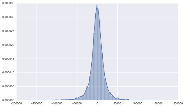
Wonderful, it’s just beautiful as we expected. And also take a look at the error of the first 5 stores.

for i in list(set(df_demand['storeid'].values))[:5]:
    value=df_demand[df_demand['storeid']==i]['diff'].values
    sns.distplot(value,bins=20)

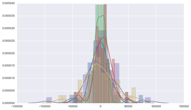
Here we comes the question: how many data points is adequate to estimate distribution? The rule of thumb is the more data you have, the better. In most cases, to get reliable distribution fitting results, you should have at least 75-100 data points available. It seems that to cluster stores will be necessary.

A Detailed Examination

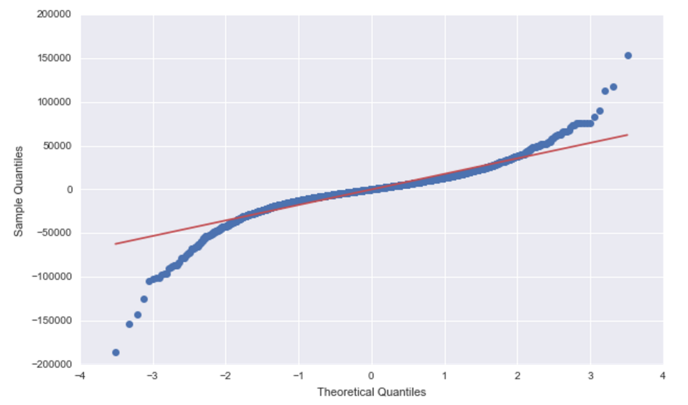
To test normality of the errors, let’s see the QQ-plot, here is a good link to understand the shape of qq-plot.

This graph is telling us that our error is still a bit heavy in the tail, that is the expected value of the normal distribution in large/small quantiles have a more tight range than the real data(why?). One possible explanation is that, some stores are newly opened s.t. they didn’t have much historical data, which makes their prediction less accurate & lot more variation.

More precise tests like Shapiro-Wilk / Kolmogorov-Smirnov are also needed:

ks_results = scipy.stats.kstest(df_demand['diff'], cdf='norm')
matrix_ks = [
    ['', 'DF', 'Test Statistic', 'p-value'],
    ['Sample Data', len(df_demand['diff']) - 1, ks_results[0], ks_results[1]]]
ks_table = FF.create_table(matrix_ks, index=True)
py.iplot(ks_table, filename='ks-table')

matrix_sw = [['Store_id', 'DF', 'Test Statistic', 'p-value']]
for i in list(set(df_demand['storeid'].values))[:10]:
    shapiro_results = scipy.stats.shapiro(df_demand[df_demand['storeid']==i]['diff'])
    shapiro_results
    matrix_sw.append(
        [i, len(df_demand[df_demand['storeid']==i]['diff']) - 1, shapiro_results[0], shapiro_results[1]])
shapiro_table = FF.create_table(matrix_sw, index=True)
py.iplot(shapiro_table, filename='shapiro-table')

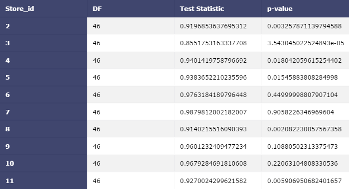
First 10 stores’ test results, we may reject them because of the lack of data. Warning: Clustering Needed.

Density Estimation

KDE will be our tool for this task. Take a look at what the cdf will look like.

df_demand['diff']=df_demand['actual_sales']-df_demand['sales_manageradj']
sns.kdeplot(df_demand['diff'].values, cumulative=True)

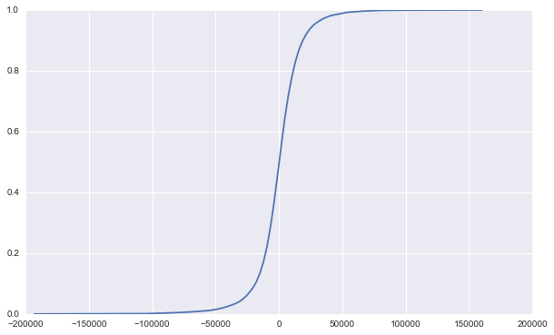
Use scipy to calculate the CDF value for a certain point given the kde.

v=10000
X=np.array(df_demand['actual_sales'].values)
gkde=stats.gaussian_kde(X)
gkde.integrate_box_1d(0,v)